Doing statistics with big data
Statistics with Big Data
- Some challenges in standard data analysis methods.
- Some solutions.
- Estimating error.
- Resampling.
- The Jackknife.
- The Bootstrap.
- The curse of dimensionality.
Big data
Data can be “big” in two different ways:
- Many rows in the table (large \(n\)).
- Many columns in the table (large \(p\)).
- Both of these present statistical challenges.
- A lot of attention has been put on large \(n\) as a solution to Reproducibility challenges.
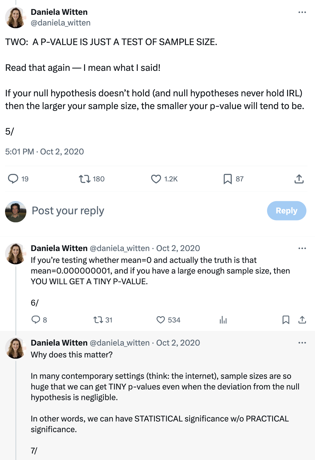
What’s wrong with NHST?
- \(H_0\) is wrong by definition
- Rejection of the null hypothesis provides very little useful information
- Type II errors are usually unquantified/unquantifiable.
- Dichotomous with fundamentally arbitrary threshold.
- Hard to use unless you restrict yourself to linear models.
The Bayesian objection
- \(H_0\) is rejected when.
- \(p(data | H_0) < 0.05\).
- But inference is often.
- \(p(H_0 | data)\) is small.
- Which may or may not be true depending on the prior of \(H_0\).
- Making \(\alpha = 0.05\) even more arbitrary.
What should we do?
- Plot the data.
- Use confidence intervals.
- If you are using ‘mixed’ factorial designs, use “within subject CIs”
- Use meta analysis.
- Use an explicit model.
- Or when pressed approximate your model with “planned comparisons”.
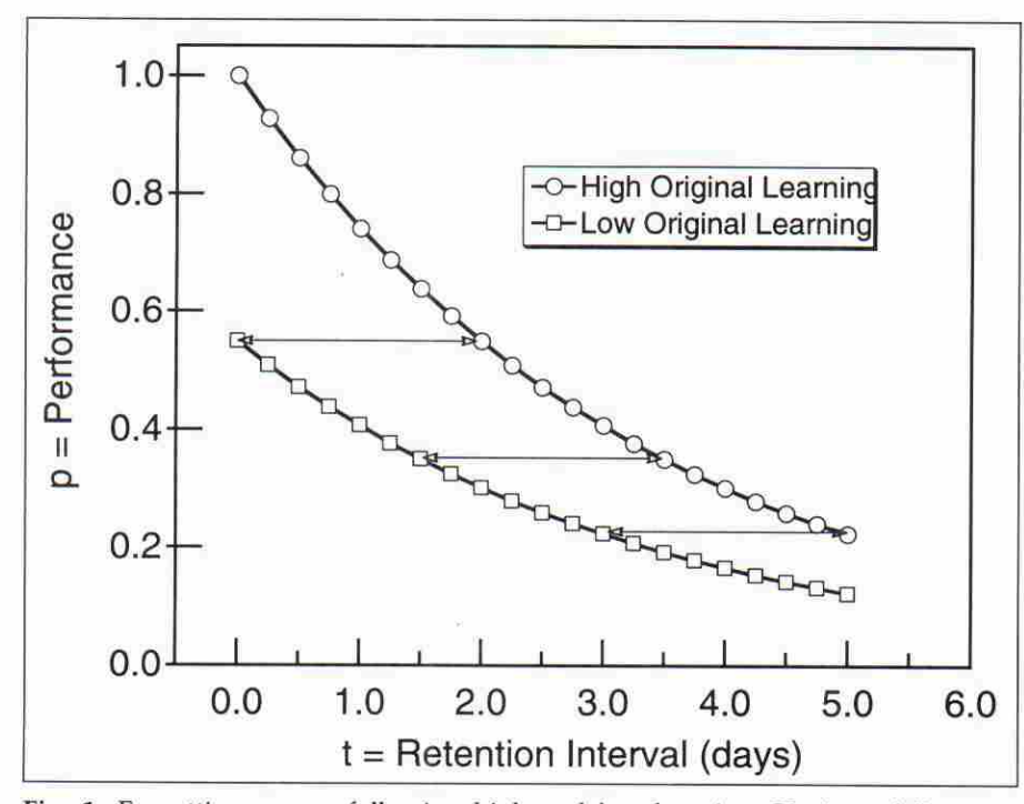
Plotting your data
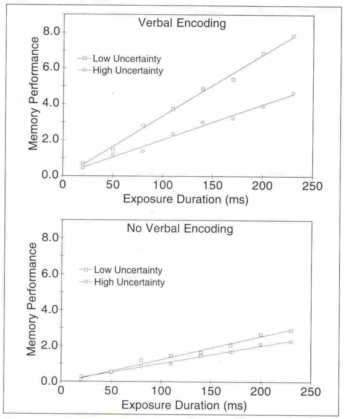
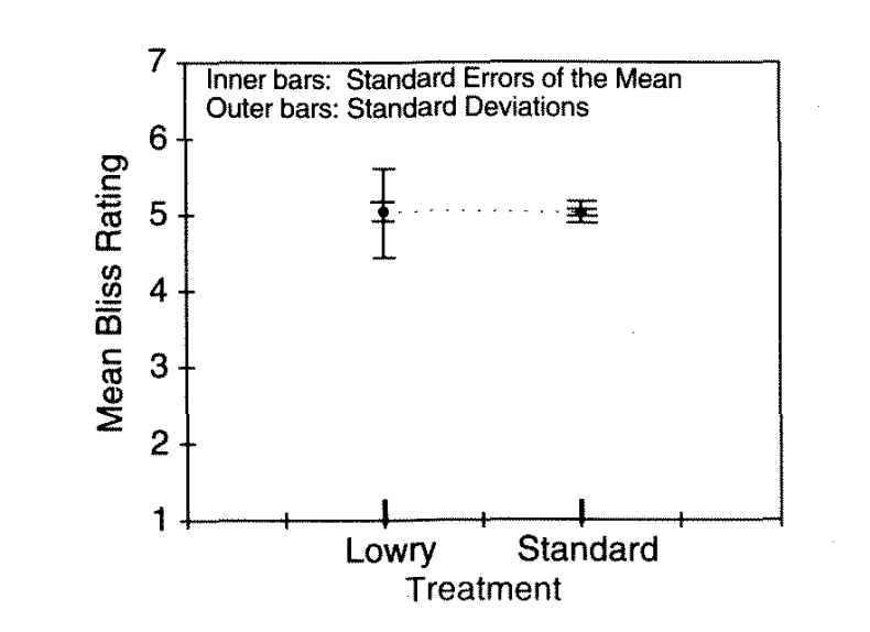
Using confidence intervals to assess results
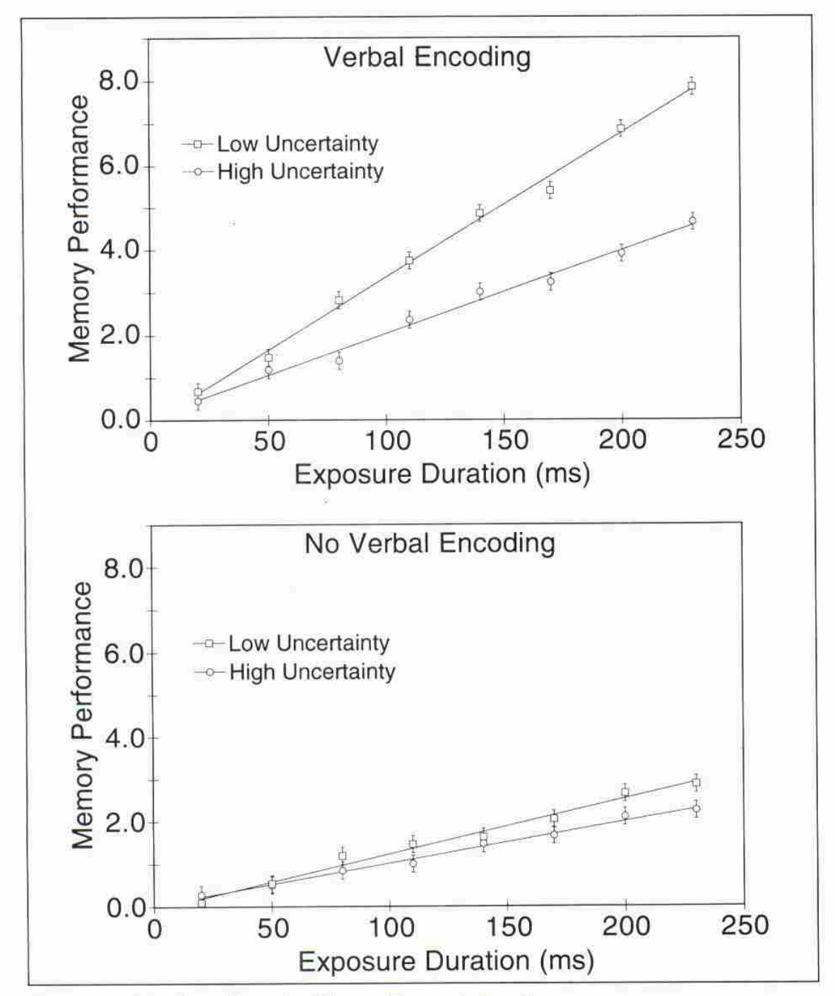
Using confidence intervals to assess results

Using confidence intervals to assess results
Explicit models
- For example, the model that Dr. Loeb used.
- Analogies from physics are useful, because physical law provides mathematical formulations of relationships.
- Or “planned comparisons”:
- Come up with a quantitative hypothesis
- Assign weights for each condition (to sum to 0)
- Compute the correlation between weights and conditional means.
Some challenges
- To calculate error bars, we need an estimate of the standard error of the statistic.
- For simple cases, this is derived from the variance of the sampling distribution.
- What is the variance across multiple samples of size \(n\).
- For some statistics (and with some assumptions), we can calculate this.
- For example, the variance of the sampling distribution of the mean: \(\frac{\sigma}{\sqrt(n)}\)
- For many statistics the sampling distribution is not well defined
- But it can be computed empirically
Computing to the rescue

Resampling methods
- Jackknife
- Cross-validation
- Permutation testing
- Bootstrapping
The Jackknife
- Originally invented by statistician Maurice Quenouille in the 40’s.
- Championed by Tukey, who also named it for its versatility and utility.
The Jackknife
- The algorithm:
- Consider the statistic \(\theta(X)\) calculated for data set \(X\)
- Let the sample size of the data be \(X\) be \(n\)
- For i in 1…\(n\)
- Remove the \(i^{th}\) observation
- Calculate \(\theta_i = \theta(X_{-i})\) and store the value
- The jacknife estimate of is:
- \(\hat{\theta} = \frac{1}{n} \sum_{i}{\theta_i}\)
- The estimate of the standard error \(SE(S)\) is:
- \(SE_\theta = \sqrt{ \frac{n-1}{n} \sum_{i}{ (\hat{\theta} - \theta_i) ^2 }}\)
The jackknife
- The bias of the jackknife is smaller than the bias of \(\theta\) (why?)
- Can also be used to estimate the bias of \(\theta\):
- \(\hat{B} = \hat{\theta} - \theta\)
Demo
Some limitations
- Assumes data is IID
- Assumes that \(\theta\) is \(\sim \mathcal{N}(\mu,\,\sigma^{2})\)
- Can fail badly with non-smooth estimators (e.g., median)
- We’ll talk about cross-validation next week.
- And we may or may not come back to permutations later on.
The bootstrap
Invented by Bradley Efron
- See interview for the back-story.
- Very general in its application
The bootstrap
- The algorithm:
- Consider a statistic \(\theta(X)\)
- For i in \(1...b\)
- Sample \(n\) samples with replacement: \(X_b\)
- In the pseudo-sample, calculate \(\theta(X_b)\) and store the value
- Standard error is the sample standard deviation of \(\theta\):
- \(\sqrt{\frac{1}{n-1} \sum_i{(\theta - \bar{\theta})^2}}\)
- Bias can be estimated as:
- \(\theta(X) - \bar{\theta}\) (why?)
- The 95% confidence interval is in the interval between 2.5 and 97.5.
Why is the bootstrap so effective?
- Alleviates distributional assumptions required with other methods.
- “non-parametric”
- Flexible to the statistic that is being interrogated
- Allows interrogating sampling procedures
- For example, sample with and without stratification and compare SE.
- Supports model fitting.
- And other complex procedures.
- Efron argues that this is the natural procedure Fisher et al. would have preferred in the 20’s if they had computers.
Demo
A few pitfalls of the bootstrap
Based on “What Teachers Should Know About the Bootstrap: Resampling in the Undergraduate Statistics Curriculum” by Tim Hesterberg.
A few pitfalls
- Estimates of SE tend to bias downward in small samples.
- By a factor of \(\sqrt\frac{n-1}{n}\)
- \(b\) is a meta-parameter that needs to be determined
- Efron originally claimed that \(b=1,000\) should suffice
- Hesterberg says at least 15k is required to have a 95% of being within 10% of ground truth p-values.
- Comparing distributions by comparing their 95% CI.
- Should compare the distribution of sampled differences instead!
- In modeling: bootstrapping observations rather than bootstrapping the residuals
- Residuals are preferable when considering a designed experiment with fixed levels of an IV.
Building on the bootstrap
- Ensemble methods:
Further reading
John Fox & Sanford Weisberg have an excellent chapter about “bootstrapping regression models” that has some excellent explanations and R code.
Another set of explanations in a Kulesa et al. tutorial paper.
The curse of dimensionality
What about large \(p\)?
- There be dragons
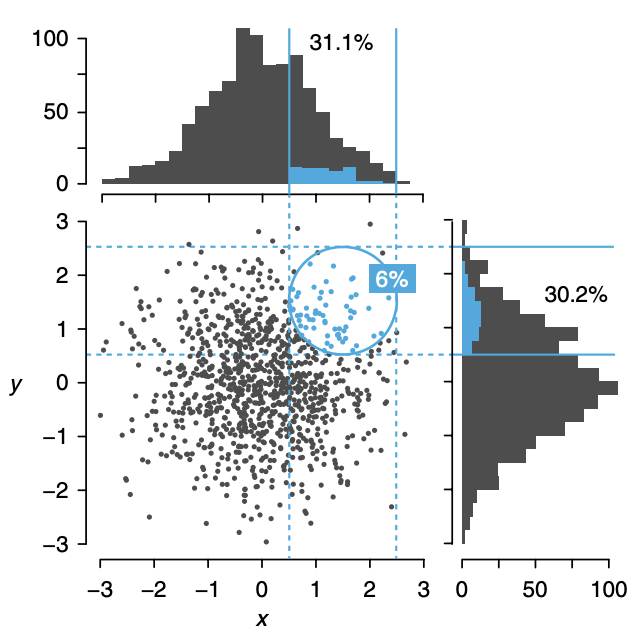
Data is sparser in higher dimensions
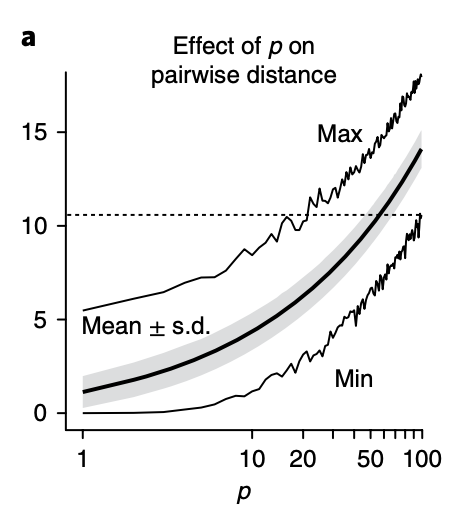
The distance between points increases rapidly
Multi co-linearity
- If the data is a \(n\)-by-\(p\) matrix:
\[ \begin{bmatrix} X_{11} & X_{12} & \cdots & X_{1p} \\ X_{21} & X_{22} & \cdots & X_{2p} \\ \vdots & \vdots & \ddots & \vdots \\ X_{n1} & X_{n2} & \cdots & X_{np} \end{bmatrix} \]
every column is a linear combination of other columns.
When \(p\) > \(n\) multi-colinearity exists
That is, there exists \(\beta\) such that
\(X_{j} = \sum{\beta_j X_{-j}}\)
But multi-colinearity can exist even when \(p\) < \(n\) !
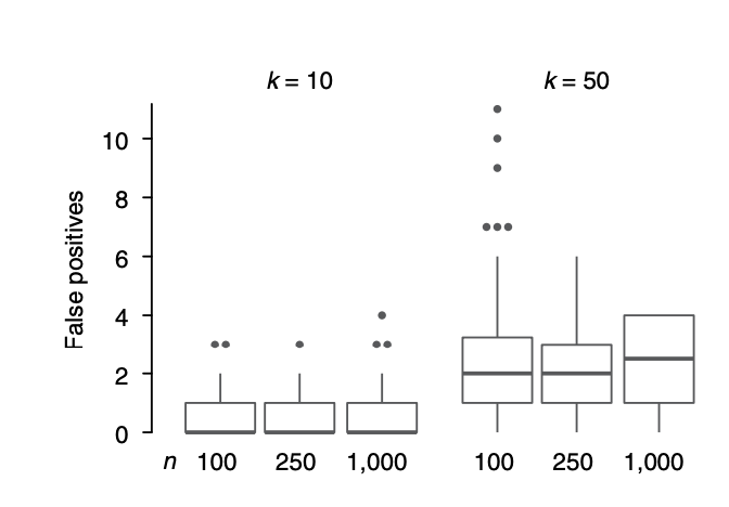
The false positive rate increases
Machine learning to the rescue?
- Next time, we’ll look at some methods that are designed to deal with the curse of dimensionality
- And may also help with some of the conceptual issues mentioned above.